Why controlling for variables is insufficient
On the pervasiveness of residual confounding in the social sciences, how to think about it, and what to do
Introduction
The aim of much social science research is to establish how things affect other things. Suppose we consider the statistical association between X and Y. This association is said to be confounded if the association is being caused by a ‘lurking’ variable (a confounder) affecting both X and Y. If we wish to estimate the total causal effect of X on Y, confounders (unlike mediators and colliders) must be controlled for.
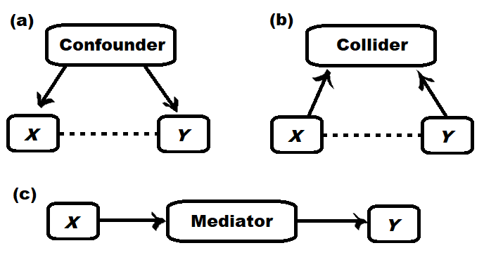
Regression analyses are widely used in the social sciences to estimate associations between variables, while controlling for other variables. It would seem then, to attain the causal effect, all we need to do is to control for confounding variables in a regression analysis. In practice, it’s more challenging than that. Particularly in the social sciences, where outcomes are affected by a large number of co-varying variables, which are often poorly measured.
This piece discusses why “controlling” for confounding variables in a regression model is insufficient to account for confounding in practice. I will give several real-world examples. Further, I will discuss how to think about confounding more broadly, and some methods for properly addressing confounding.
Why adjusting for confounding is insufficient
A common approach in regression analysis is to attempt to isolate the effect of an exposure on an outcome by controlling for the other important variables. One way to illustrate the inadequacy of this approach is by comparing observational studies with experimental results. The results are sobering.
Consider, for example, one study analyzing the performance or “value” of various health plans (Wallace et al., 2022). The basic issue is that people may select non-randomly into different health plans, creating spurious associations between health plans and performance indicators. Thus, researchers have attempted to control for confounding variables. But was this sufficient? No. By comparing random allocation estimates from the observational adjusted estimates, residual confounding remained substantial in the observational studies.
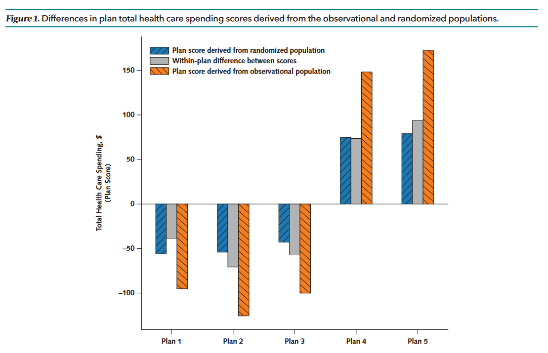
There are two reasons why residual confounding can be so persistent:
Omitted variable bias. Important variables may be missing in the regression analysis. It is often not practically feasible to account for all practically relevant variables. Some effects (e.g., genetics) may not even be feasible to measure directly in individuals.
Included variables only partially controlled. A different issue is that even variables included in the analysis may not be fully controlled away. Measurement error is a common reason. In the social sciences, measurement error is often substantial, and, in those cases, controlling for X (the measurement) only partially adjusts for X (the actual construct of interest). The equivalent is the case is if the observed variable is only a proxy of the actual construct of interest. A second way is if the relationship between the variable and outcome is not modeled correctly. For example, if linear regression is used but the relationship is not linear, or simply if parameters in the regression are not estimated well due to insufficient data. In those cases, there may also be residual confounding.
While most will understand these points in the abstract, I think many do not sufficiently appreciate the extent to which it matters. Beyond the example I have already given, many other examples confirm that causal effects are often not well-estimated in observational studies.
A different study looked at effect of digital advertising (Gordon et al., 2018). Again, they compared randomized experimental studies with observational research, and concluded: “the observational methods often fail to produce the same effects as the randomized experiments, even after conditioning on extensive demographic and behavioral variables.”
Similarly, Wilde & Hollister (2007) find that propensity score matching compares poorly to experimental research when estimating the effect of classroom size on achievement test scores.
One of the more shocking examples is by Eckles & Bakshy (2021). They looked at a huge high-dimensional dataset, evaluating peer effects on behavior. They concluded that: “Compared with the experiment, naive observational estimators overstate peer effects by over 300% and commonly available variables (e.g., demographics) offer little bias reduction.” They had to use 3,700 predictors to reduce bias to non-significance.
In short, substantial residual confounding is usually present and often substantial, even after controlling for an extensive set of measured confounders.
The impact of measurement reliability
As noted previously, one contributor to residual confounding is the effect of omitted variables. A second issue is that effects of included variables are not entirely removed, for instance when variables are imperfectly measured. This section will explore the latter issue.
Example 1: the grandparent effect
In an excellent paper, Engzell et al. (2020) demonstrated how these problems can manifest in practice. While the statistical points have relevance in many contexts, the specific question they asked was: what is the role of grandparents in social status transmission across generations? That is, do the grandparents’ social status matter net of that of the parents?
First, as you might have predicted following the previous section, they found that even an extensive set of parental socioeconomic controls was insufficient to account for parental confounding. In particular, they found that parental cognitive ability was still a confounder beyond the socioeconomic controls.
Next, they wondered how the magnitude of residual confounding would depend on the quality and richness of the control variables. The researchers had access to detailed, reliably measured data from Swedish population registries — better quality data than researchers typically have access to in their analyses. But what if the data quality was poorer? To answer this question, they simulated their control variables to be less comprehensive and of lower quality in ways often seen in the literature. They (a) changed the number of parental socioeconomic indicators they used as controls (among parental education, occupation, and income); (b) changed how detailed each variable is operationalized, for example by putting earnings into bins instead of using the actual value (e.g., one bin being $15,000-$20,000; another being $25,000-$30,000, etc); (c) lastly, they introduced artificial measurement error of varying sizes.
The quality of the controls had a massive impact on the estimated grandparent “effect.” The smallest estimate was reached with the highest quality controls. But, in most of the simulations, the grandparent coefficient more than doubled and, in the absolute worst cases, quadrupled.
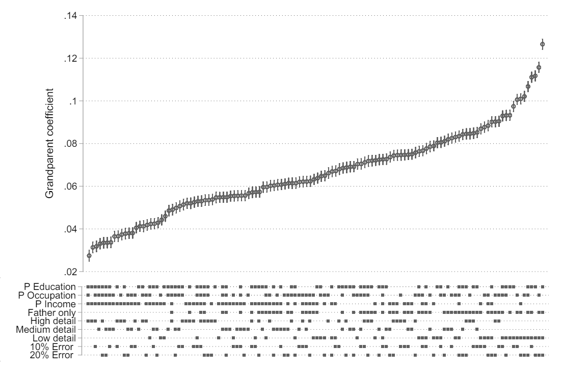
In short, the issue of residual confounding is greatly exacerbated when the set of control variables less comprehensive, less detailed and/or less accurately measured.
Example 2: genetic confounding and polygenic score controls
Another common major source of confounding is genetics. Nearly all human traits are heritable, meaning a nonzero fraction of the variation in those traits can be attributed to genetic differences.
The genetic influence on some trait within an individual can be captured to some extent with so-called polygenic scores (or risk scores, indices, etc). Many researchers have jumped on this opportunity to use polygenic scores to “control” away the genetic influence on a particular trait away.
Unfortunately, this is yet another example where statistical adjustments are insufficient. Polygenic scores can be seen as measurements of genetic influence, but only with substantial measurement error. While genotyping itself can be done with high reliability, the estimation of genetic influence from genotype still suffers from misestimation. Polygenic scores only capture a modest portion of heritability for most traits, thus they are inadequate as statistical controls (Zhao et al., 2024). Unmeasured genetic confounding is therefore expected to be substantial even after such controls.
How much confounding remains? — Discrimination and disparities
The coefficient after adjusting for measured confounders is often interpreted as the causal effect. But when estimating an effect in a regression analysis, we should ask ourselves how much residual confounding is likely to persist. Even if our thoughts are initially based largely on intuition, it is an important consideration. In this section, I will consider this question in the context of discrimination and group disparities, where residuals have often been interpreted as discrimination.
When we find disparities between groups — whether it’s gender wage disparities, racial disparities in the criminal justice system or any other disparity — there is always the question of discrimination. How much, if any, of the disparity can be blamed on discrimination?
Regression analyses have been widely applied to address such questions. There is an intuitive appeal of this approach: control for the relevant variables, and the remaining disparity reflects discrimination. But the careful reader will notice the issue immediately. There will invariably be omitted-variables bias, and even variables that are included in the regression analysis are only imperfectly controlled away (e.g., due to measurement error or imperfect modelling of variable relationships). Thus, we cannot infer that the residual reflects discrimination.
The question is then, when can we reasonably infer a causal effect? In this context, when does a disparity reflect discrimination? And where is it plausible that the disparity could be accounted for by other relevant variables?
Example: racial discrimination in Harvard admissions
A number of years ago, a lawsuit was filed against Harvard alleging that the undergraduate admission practices were racially discriminatory. Consequently, detailed admissions data was released and a number of in-depth statistical analyses of the university’s admission process were conducted.
If one naïvely looked at the crude admission rates by race, there would be no huge disparities, and perhaps little indication of discrimination.1 But of course, we should consider the most relevant confounders. First and foremost, academic credentials.
When we control for academic credentials, the disparities markedly increase. That is, the racial disparities in admit rates for academically equivalent students (controlled) are much larger than the racial disparities in the entire applicant pool (crude). The figure below illustrates this comparison. This is unusual (though not unheard of), as controlling for the most relevant confounders typically reduces disparities.
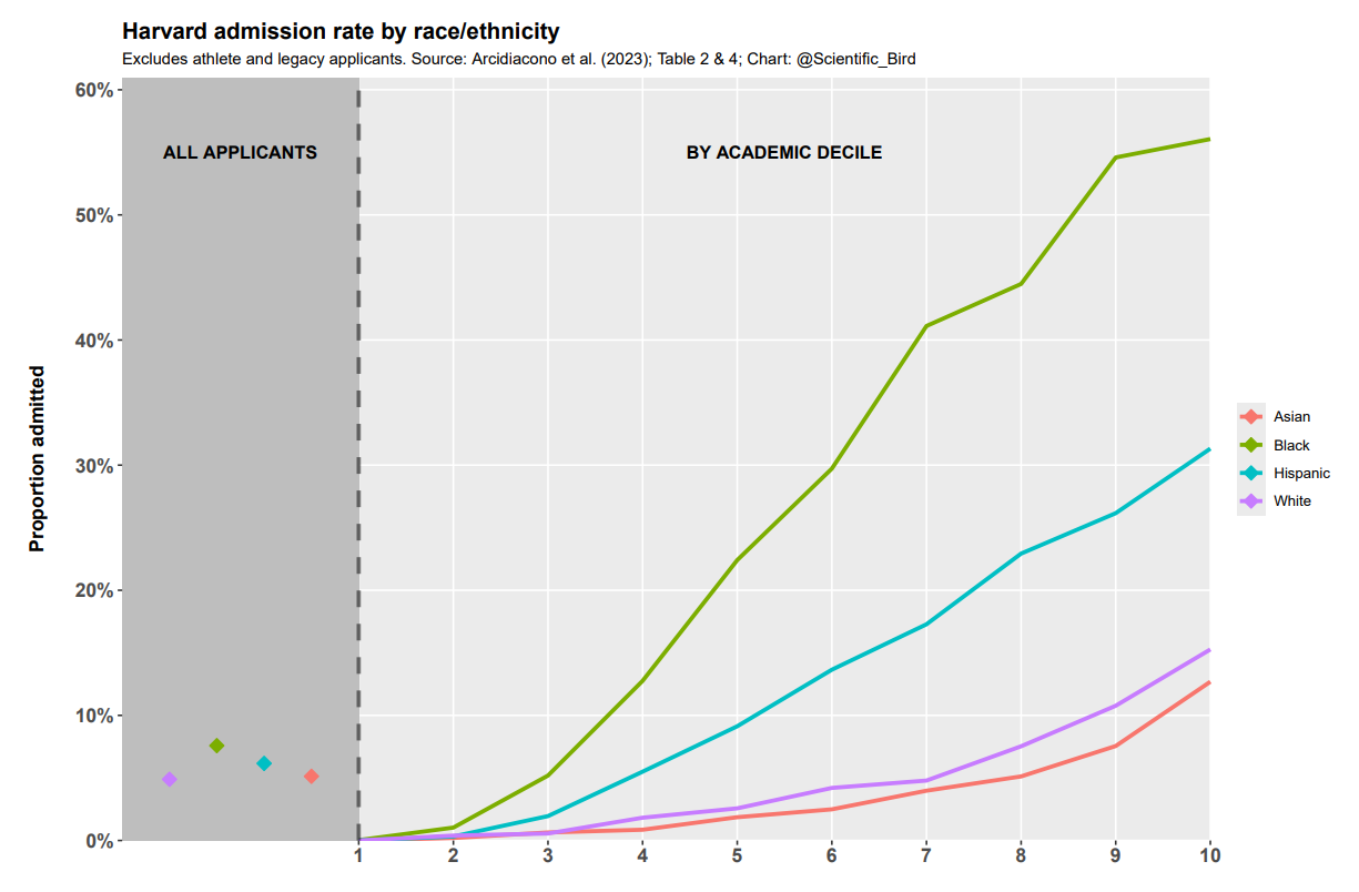
The disparities were very large. A black applicant with academic credentials just a little below the typical applicant was substantially more likely to be admitted than a white or Asian applicant with academic credentials in the top decile (22.4% black applicants in 5th decile; 15.3% and 12.7% for white and Asian applicants in the 10th decile, respectively). In the top decile, a black applicant was many times more likely to be admitted than a white or Asian applicant.
It was argued by some (e.g., David Card who testified on behalf of Harvard) that residual confounding might account for the observed disparities. That is, something other than what’s captured in the academic indices is responsible for the disparities.
But we must always distinguish between theoretical possibility and plausibility in practice. The argument strains credulity as it implies something highly improbable about the direction and, in particular, the magnitude of residual confounding.
First, direction. As noted, when we control for the best measures of academic credentials (SAT, grades, etc), the admission gaps become larger, not smaller. Generally, residual confounding is expected to be in the same direction as observed confounding, and, in humans, positive educational traits tend to go together. Thus it is more likely that perfect (non-discriminatory) controls would further increase the gaps rather than diminish them.
Second, magnitude. Any such hidden variable hypothesized to account for the gaps has to be of implausibly large importance. As noted, the gaps in admission rates for individuals of similar academic credentials were huge. Such a hidden variable would need to have about equal (and independent) explanatory power of all the measures of academic credentials put together (e.g., grades and SAT score). But no such candidate variables are even known in the literature. Not only that, Arcidiacono et al.’s model for predicting admissions was high, leaving little room for unobserved factors to be so influential they would need to be. We are firmly entering the territory of practical impossibility.
In short, the gaps became larger as the most relevant variables were taken into account. The gaps were in the opposite direction of what you would expect had they been caused by non-discrimination. Most importantly, the adjusted disparities were far too large for them to plausibly be explained by unmeasured non-discriminatory variables. It was a straightforward case of discrimination. The court agreed, and it was ruled that Harvard’s admissions practices had been racially discriminatory and unconstitutional.
Disparities, discrimination and residual confounding
To infer discrimination from any disparity would be a mistake, however. The Harvard case was special: controlling for the most relevant confounders increased the gaps rather than decreased them, and the size of the adjusted disparities were simply too large to plausibly be explained by non-discriminatory residual confounding.
In many other scenarios, however, controlling for the domain-relevant confounders diminishes the gaps, and the adjusted disparity is small enough that residual confounding could plausibly account for remainder of the gap.
The most obvious example is the gender wage disparity. According to one analysis, the unadjusted disparity is 17% and the adjusted disparity is just 1%. Because the adjusted gap is so small, we cannot reject the possibility that residual confounding could account for the rest. It is fallacy to suggest (as the authors do) that the adjusted residual “should be zero.” Residual confounding, due to omitted variables and/or imperfectly controlled variables (e.g., due to measurement error), is to be expected.
A complication is that, as mentioned in the introduction, controlling for some variables (mediators and colliders) can bias the estimate of the causal effect of discrimination. One argument is that (for example) occupation is itself affected by discrimination, and thus adjusting for occupation controls away one mediator of discrimination, underestimating its effect. That is a different issue, and this is not the place to settle this debate. Rather, the point is just that the regression results alone are compatible with a plausible non-discrimination story, unlike the Harvard case.
A second example is racial disparities in the criminal justice system. For example, Rehavi & Starr (2014) use quantile regression to analyze black-white disparities in federal sentencing length. They find that most of the sentencing length disparity can be accounted for by legally relevant confounders. Controlling for observed confounders reduced the median log sentence gap from 0.721 to 0.087 (Q50, Table 3). In other words, 88% [1 - 0.087/0.721] of the disparity was accounted for by observed legally relevant differences. Many would be quick to attribute the rest to discrimination, but the authors do recognize that other explanations are possible. A priori, we should always expect that controlling for observed variables only partially accounts for confounding. Because the unexplained portion is so small relative to the explained portion, it is well within the realm of practical plausibility that a hypothetical perfect set of controls could account for 100% of the disparity. Again, the issue is that it’s impossible to measure all relevant variables (including relevant unobserved defendant characteristics), and even measured variables will never perfectly control for the actual constructs of interest (e.g., any quantification of offense type, offense severity, and offense history will inevitably be somewhat coarse and miss the finer distinctions between offenses).
A recent study helped settle the question regarding racial discrimination in the American criminal justice system (Hoekstra et al., 2023). The researchers exploited quasi-random assignment of cases to grand juries, eliminating systematic error arising from omitted-variables bias. By far the largest study of its kind, they concluded that “grand jurors do not engage in statistical or taste-based discrimination against Black defendants.”
As a general matter, whether the entire residual can plausibly be attributed to confounding is not always easy to assess. Clearly we should refrain from prematurely concluding that a residual must be discrimination. In some scenarios, sensitivity analyses can help estimate the magnitude of the residual confounding component (e.g., Bollinger, 2003). But ultimately, the best solution is to use a research design which accounts for unobserved confounding.
Addressing unobserved confounding
If we want to estimate the (average) causal effect, we need to eliminate systematic differences affecting the outcome, which would otherwise contaminate our comparisons. As we have seen, nontrivial confounding often remains even with extensive controls. Measured controls are simply insufficient. We need a research design which, by construction, accounts for unmeasured confounding (see, e.g., D’Onofrio et al., 2013; Duncan et al., 2004; Munafò et al., 2021).
As discussed earlier, the classical approach is the randomized controlled trial. But conducting these is not always practically feasible. The so-called “credibility revolution” in econometrics has led to more widespread usage of quasi-experimental methods which are better suited to estimate causal effects in observational data. Examples include: instrumental variable estimation, regression discontinuity designs, difference-in-difference estimation, among others. All these methods have their advantages and disadvantages, and are more applicable in some contexts than in others. To review all such methods could easily fill an entire book.2 Instead, in the final section I will explore one example of a research design used to explore causal questions from observational data.
Example: maternal smoking during pregnancy and offspring outcomes
One method used to account for unobserved confounding is the sibling discordant exposure design. It compares siblings within families, who nevertheless were differentially exposed to a certain variable. By construction, it controls for anything the siblings share, whether measured or not.
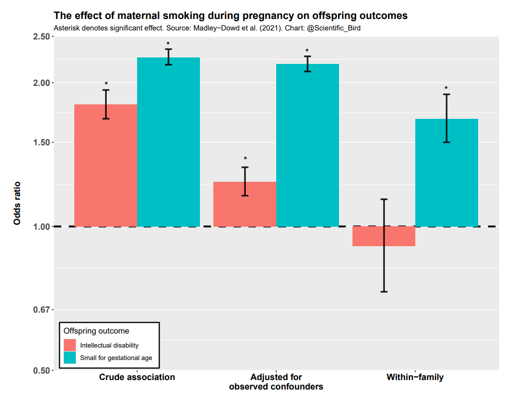
An example of this research design being applied was to test the effect of maternal smoking during pregnancy on offspring outcomes (Madley-Dowd et al., 2021). That is, to account for unobserved confounding, they compared siblings (within-family) where the mother smoked only while pregnant with one of them.
The results of their analysis are summarized below. The crude associations, the associations adjusted for observed confounders, and finally the within-family (sibling difference) associations are all shown. Two offspring outcomes — intellectual disability and birth weight — were analyzed.
For offspring intellectual disability, the association with maternal smoking was significant without controls and when measured confounders were controlled for, but not when unobserved confounders were controlled for (in the within-family approach). This means that, had we stopped at the usual stage after controlling for observed confounders, we would’ve been misled to think there was a significant effect. In reality, there appears to be no causal effect of maternal smoking on offspring intellectual disability.3 On the other hand, the association with low birth weight was significant and substantial even in within-family comparisons, consistent with a causal interpretation. The most plausible explanation is that smoking while pregnant does affect the physical development of the fetus, even if not necessarily psychological development.
Researchers have used the same research design to assess the effect of maternal smoking during pregnancy on offspring ADHD (Skoglund et al., 2014; Obel et al., 2011; Obel et al., 2016). The figure below summarizes the results from three large Nordic studies. In none of the countries is the association significant between siblings within families. Again, the causal effect of maternal smoking on this psychological outcome appears minimal or null.
In summary, maternal smoking during pregnancy does appear to affect the physical growth of the fetus, but the psychological effects analyzed are minimal.4
Conclusion
In this piece, I have argued that residual confounding is a widespread and serious issue in the social sciences. Comparisons between observational and experimental research show that even rich sets of control variables are insufficient to account for confounding. Furthermore, I have shown that this issue is greatly exacerbated when control variables are lacking in detail or are not well measured, as is commonplace in the social sciences.
In general, it is thus not sufficient that an effect persists after controlling for confounders to infer that it is a causal effect. As example, I have looked at studies where the adjusted residual between groups is often interpreted as discrimination. Because meaningful residual confounding is the norm, this inference is often unjustified (except in specific cases, e.g., where the adjusted disparity is too large for residual confounding to be a plausible explanation).
Experimental research is generally considered the cure to this problem, but it is not a cure we always have access to. I am a proponent of using research designs which, by construction, account for important sources of unmeasured confounding. I have used the example of maternal smoking on birth weight as an example, where the discordant sibling design results are at least consistent with a causal interpretation. Triangulating this with compelling results from other research designs, we can be even more confident that this interpretation is correct. In practice, that is probably the best we can do.
I am not suggesting that adjusting for variables should never be done, or that anything that isn’t “perfect” should be rejected. We cannot formally prove scientific results in the same way mathematicians can. All we can do is inference to the best explanation. But, even acknowledging these pragmatic realities, the social sciences have definitely suffered due to insufficient attention to residual confounding. Addressing this would be an important step forward to reaching more reliable conclusions about causality.
In fact, Arcidiacono et al. (2022) have shown that “Harvard encourages applications from many students who effectively have no chance of being admitted, and that this is particularly true for African Americans.” The racial bias in the unadjusted admission rates was thus masked by the inclusion of students who had no chance of being admitted, so Harvard could admit other students (who would not have been admitted absent preferences).
A good book that deals with the subject in an approachable and easy-to-follow way is Mastering ‘Metrics by Angrist and Pischke.
It is true that the persistence of an effect within families is not 100% proof of a causal relationship. The most pressing concern is if sibling differences confound the relationship between exposure and outcome. Suppose you want to know whether divorce causes suicide. A sibling difference in divorce (exposure) might be confounded by various sibling differences responsible for both divorce and suicide (e.g., differences in mental health). But in our maternal smoking example, as the exposure affects them before they are even born, this is less of a concern. Furthermore, while I have just discussed one research design, the proposition that maternal smoking affects birth weight is supported by a wide range of other research designs (see textbox 3, Krieger & Smith, 2016). Thus, it is most reasonable to conclude (based on the weight of the evidence) that there is a causal effect of maternal smoking on birth weight.



This is an excellent article, but I find it a little too credulous regarding quasi-experimental designs. See e.g.
Wei Jiang, Have Instrumental Variables Brought Us Closer to the Truth, The Review of Corporate Finance Studies, Volume 6, Issue 2, September 2017, Pages 127–140, https://doi.org/10.1093/rcfs/cfx015
Maybe I haven't read carefully enough, but I want to add another problem that I didn't see here: Causality in the other direction. For example, I've seen multiple papers in which an association between poverty and some negative trait was tested, such as low intelligence, and when they got the unsurprising result that these two are associated, they immediately state that this proves poverty causes the negative trait. However, it should be obvious that there is a wide range of negative traits that would adversely impact your monetary situation, by reducing income and/or by increasing wasteful spending.